plot2 for ggplot2 users • plot2

library(plot2)
library(ggplot2)
library(dplyr)

This article is for users who know ggplot2. It describes how the concepts of plot2() relate to those of ggplot2, and what plot2() does by default.

Concepts

ggplot2 builds a plot from components: data, aesthetic mappings, geoms, statistics, scales, coordinates, facets and a theme. plot2() builds the same components, but its arguments describe the plot instead of the components:

`plot2()`	`ggplot2`
`x`, `y`	`aes(x = , y = )`
`category`	`aes(colour = )` or `aes(fill = )`, depending on the geom; or another aesthetic set with `category.type`
`facet`	`facet_wrap()`
`type`	`geom_*()`, together with the position, such as `position_dodge()`
calculations in `x`, `y`, `category` and `facet`	`group_by()` and `summarise()` or `mutate()` before the plot
`x.sort`, `category.sort`, `facet.sort`	`forcats::fct_reorder()`, `fct_infreq()` or `fct_relevel()` before the plot
`x.max_items`, `category.max_items`	`forcats::fct_lump_n()` before the plot
`colour`, `colour_fill`	`scale_colour_()` and `scale_fill_()`
`x.` and `y.` settings	`scale_x_()` and `scale_y_()`
`datalabels`	`geom_text()` or `geom_label()` with the summarised values
`title`, `x.title`, `category.title`, …	`labs()`
`theme`	`theme_*()` and `theme()`

An example

This plot shows the number of admissions per hospital and gender, sorted by the total number of admissions, with data labels. In ggplot2, the data are summarised and sorted first:

admitted_patients |>
  count(hospital, gender) |>
  mutate(hospital = reorder(hospital, -n, FUN = sum)) |>
  ggplot(aes(x = hospital, y = n, fill = gender)) +
  geom_col(position = position_dodge(width = 0.6), width = 0.5) +
  geom_text(aes(label = n), position = position_dodge(width = 0.6), vjust = -0.5) +
  scale_y_continuous(expand = expansion(mult = c(0, 0.1))) +
  labs(x = "Hospital", y = "Admissions", fill = "Gender") +
  theme_minimal()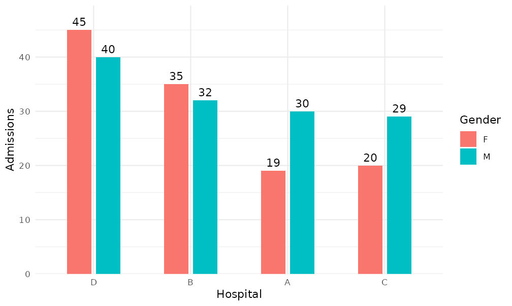

In plot2(), the same steps are arguments:

admitted_patients |>
  plot2(x = hospital,
        y = n(),
        category = gender,
        x.sort = "freq-desc",
        x.title = "Hospital",
        y.title = "Admissions",
        category.title = "Gender")
#> Applying x.sort = "freq-desc" using summarise_function = sum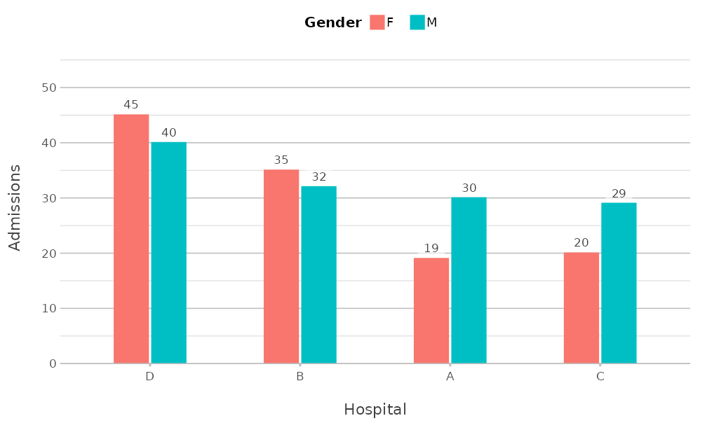

The results differ in style, because each package has its own defaults; the next section lists those of plot2().

Defaults of plot2()

plot2() sets these defaults, each of which can be changed with the argument concerned:

The theme is theme_minimal2() (argument theme; theme = NULL uses the default theme of ggplot2).
The y axis starts at zero where possible and has extra room at the top (y.zoom, y.limits and y.expand).
Column plots have data labels when there are at most 25 columns (datalabels).
The legend is at the top, or at the right for a numeric category (legend.position).
Text and factor values of x are sorted alphabetically, with numbers in their numeric order (x.sort).
Whole numbers that look like years or months become text in discrete plot types (x.character and category.character).
Large and small numbers on the y axis are formatted with a thousands separator or in scientific notation (y.scientific, big.mark and decimal.mark).
Axis titles are taken from the given columns or calculations (x.title, y.title, category.title).

The section Automatic choices in ?plot2 lists all rules, and in an interactive session plot2() reports each decision in a message.

Continuing with ggplot2

plot2() returns a ggplot object, so every ggplot2 function can be added to it:

admitted_patients |>
  plot2(x = age, type = "histogram", binwidth = 5) +
  geom_vline(xintercept = 65, linetype = "dashed") +
  annotate("text", x = 64, y = 40, label = "Aged 65 and over", hjust = 1) +
  scale_x_continuous(breaks = seq(0, 100, 10))
#> Assuming smooth = TRUE for type = "histogram"
#> Scale for x is already present.
#> Adding another scale for x, which will replace the existing scale.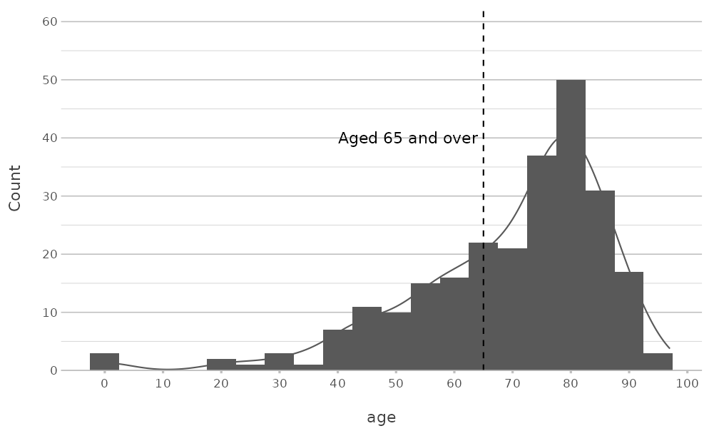

A scale that plot2() already set is replaced, with a message from ggplot2. Use the x.* and y.* arguments of plot2() to avoid this.

The package also has functions to change a plot afterwards:

add_type() adds any geom with the data of the plot, and add_line(), add_point(), add_col(), add_errorbar(), add_smooth() and add_sf() add the most common ones;
add_mapping() adds or changes an aesthetic mapping;
move_layer() changes the order of the layers;
get_plot_title() returns the title of a plot, for example to use it as a file name.

Using parts of plot2 with ggplot2

Several functions of plot2 also work in plots made with ggplot2 alone:

theme_minimal2(), the theme;
coord_spider(), the coordinate system of spider plots;
get_colour(), which returns colours from palettes and registered colours, for example for scale_fill_manual(values = get_colour("viridis", 4));
md_to_expression(), which converts markdown to a plotmath expression for titles and labels;
the labelling functions euros() and dollars(), for scales and data labels.

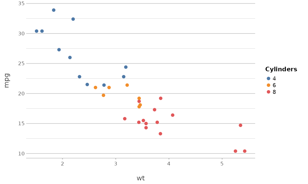
ggplot(mtcars, aes(x = wt, y = mpg, colour = factor(cyl))) +
  geom_point(size = 2) +
  scale_colour_manual(values = get_colour("Tableau 10", 3)) +
  labs(colour = "Cylinders") +
  theme_minimal2()