Colours and themes

library(plot2)

This article describes how plot2() sets colours, how to use palettes and the colours of an organisation, and how to change the theme and the titles of a plot.

Setting colours

colour sets the colours of a plot, whatever its type. ggplot2 distinguishes between the colour aesthetic (for points and lines) and the fill aesthetic (for areas such as bars), each with its own scale functions. plot2() determines which of the two applies and sets both where needed. Without colour, the colours of ggplot2 are used:

admitted_patients |>
  plot2(x = hospital, y = n(), category = ward)

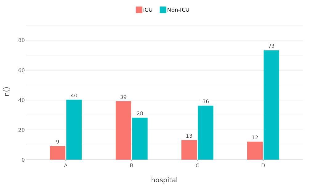
colour accepts R colour names, hexadecimal codes and palette names. A vector of colours is used in the order of the values of category:

admitted_patients |>
  plot2(x = hospital, y = n(), category = ward, colour = c("steelblue", "#E15759"))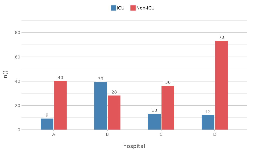

A named vector matches its names to the values of category, so that a value keeps its colour in every plot, even when not all values are present:

admitted_patients |>
  plot2(x = hospital,
        y = n(),
        category = ward,
        colour = c("Non-ICU" = "grey70", "ICU" = "#E15759"))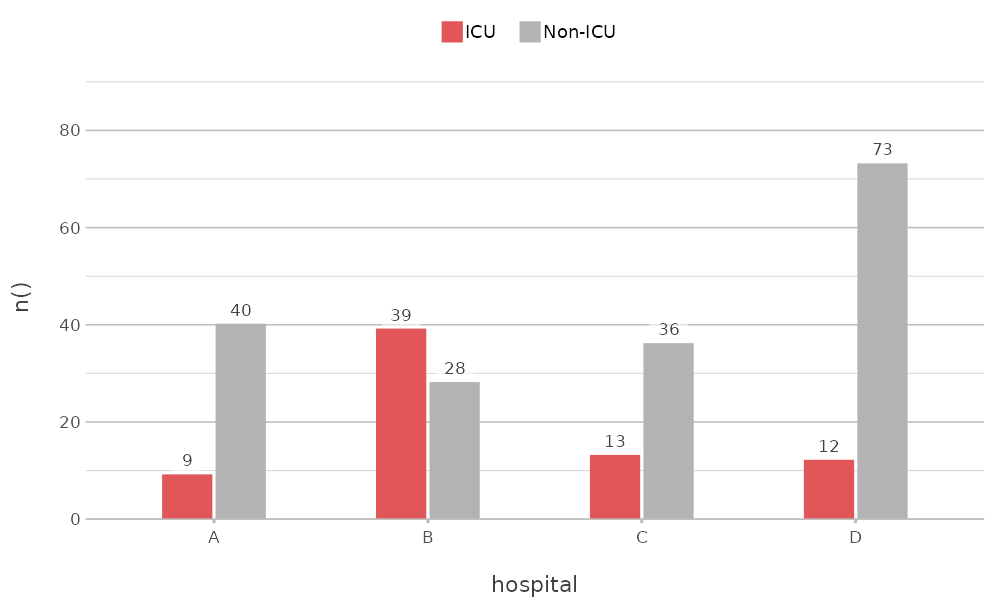

Palettes

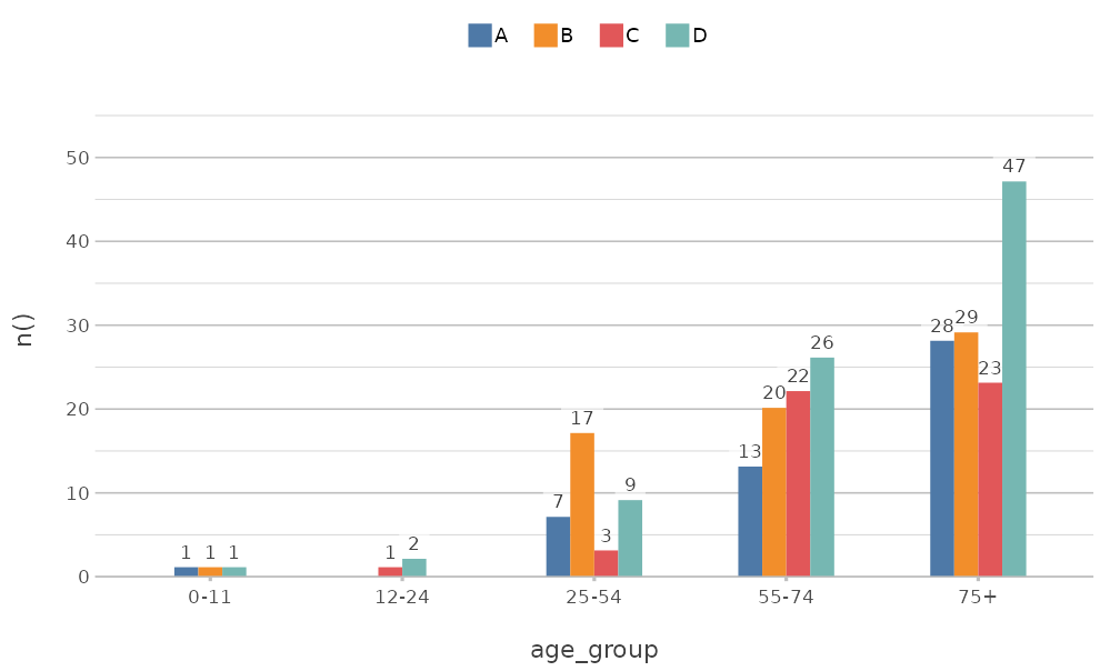
The colourblind-safe palettes of the viridisLite package are available by name: "viridis", "magma", "inferno", "plasma", "cividis", "rocket", "mako" and "turbo". So are the palettes of base R, such as "Okabe-Ito", "R4" and "Tableau 10" (see grDevices::palette.pals()):

admitted_patients |>
  plot2(x = age_group, y = n(), category = hospital, colour = "Tableau 10")

get_colour() returns the colours that plot2() uses for a name or palette. A palette is extended where needed, so that it never runs out of colours:

get_colour("Tableau 10", length = 4)
#> [1] "#4E79A7"  "#F28E2B"  "#E15759"  "#76B7B2" 
get_colour(c("red", "#4E79A7", "f80"))
#> [1] "#FF0000"  "#4E79A7"  "#FF8800" 

Colour and fill

Where a geom has both a line and an area, such as columns and boxplots, colour applies to both. colour_fill sets the area separately:

admitted_patients |>
  plot2(x = hospital,
        y = age,
        category = ward,
        type = "boxplot",
        colour = c("#4E79A7", "#E15759"),
        colour_fill = "white")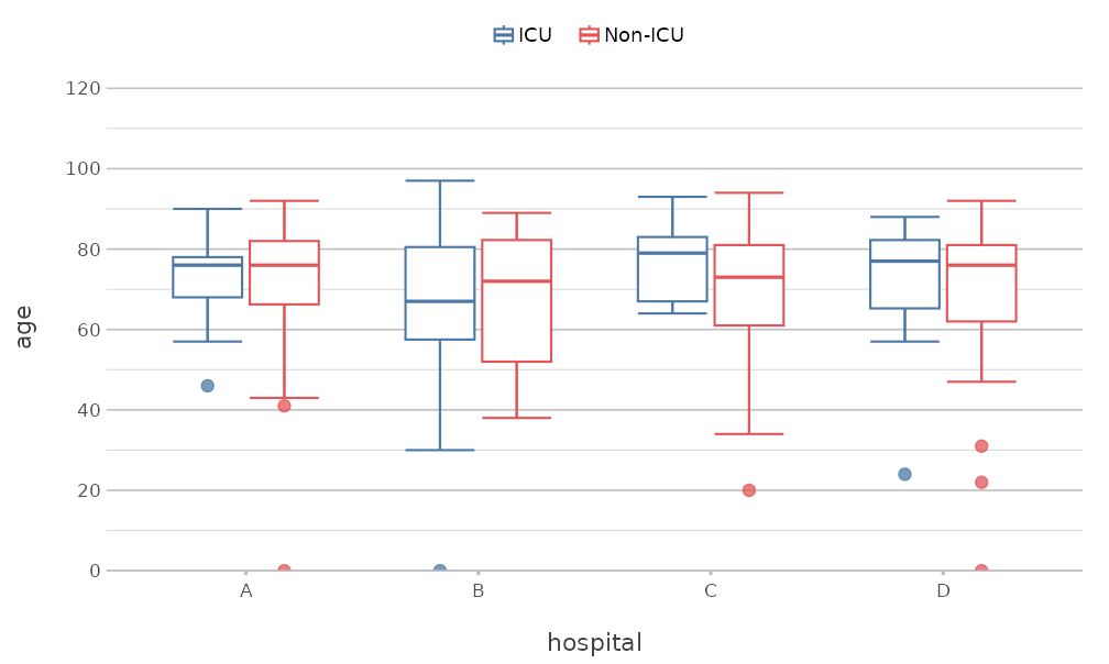

colour_transparency makes the colours transparent, from 0 (solid) to 1 (fully transparent).

Numeric categories

A numeric category gets a continuous colour scale. Two colours give a gradient, and three colours give a scale that diverges from the midpoint, which category.midpoint sets:

mtcars |>
  plot2(x = wt,
        y = mpg,
        category = hp,
        colour = c("#2166AC", "grey90", "#B2182B"),
        category.midpoint = 150,
        size = 3)
#> Using type = "point" since both axes are numeric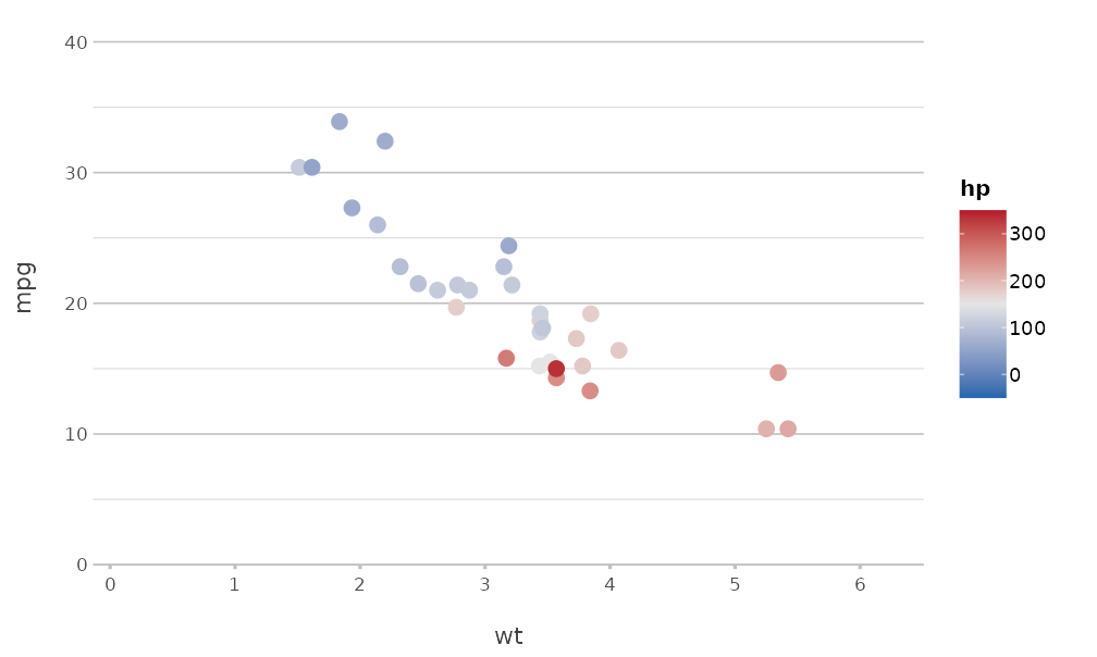

Highlighting a value

category.focus shows one value in its colour and the other values in grey. It accepts a value or its position:

admitted_patients |>
  plot2(x = format(date, "%Y"),
        y = n(),
        category = hospital,
        category.focus = "D",
        type = "line",
        x.title = "Year")

Colours of an organisation

register_colour() adds colours under a name of your choice, which can then be used everywhere plot2() accepts colours. A set of registered colours can itself be registered as a palette:

register_colour(company_blue = "#1F3A93",
                company_orange = "#D35400",
                company_green = "#2C6F47",
                company_grey = "#708090")
#> 4 colours registered.
register_colour(company = c("company_blue", "company_orange", "company_green", "company_grey"))
#> 1 colour set registered.

get_colour("company", length = 4)
#> [1] "#1F3A93"  "#D35400"  "#2C6F47"  "#708090"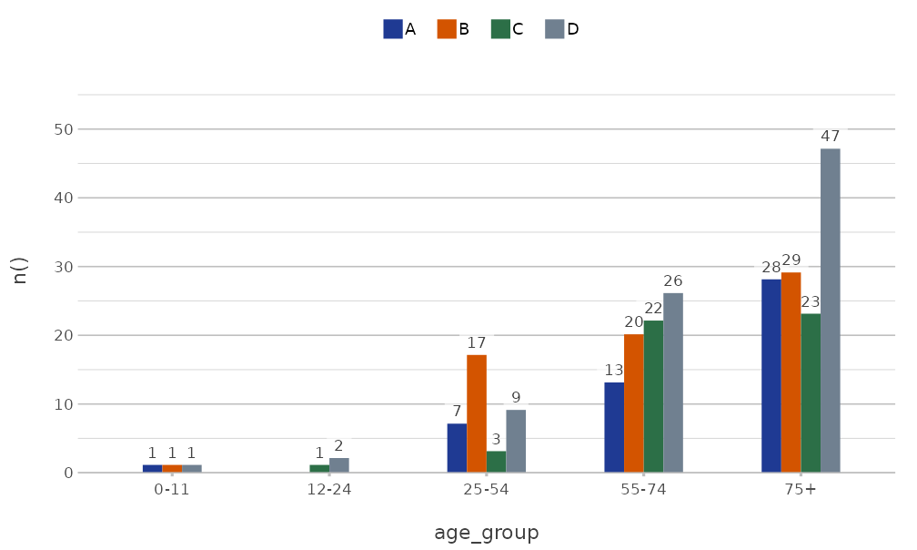 

admitted_patients |>
  plot2(x = age_group, y = n(), category = hospital, colour = "company")

The option plot2.colour sets the default colours for all plots in the session:

options(plot2.colour = "company")

admitted_patients |>
  plot2(x = hospital, y = n(), category = gender)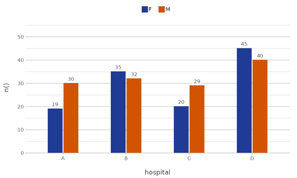

options(plot2.colour = NULL)
unregister_colour("^company")
#> 5 colours unregistered.

A package can register colours when it is loaded, so that all users of that package get the same colours. ?get_colour shows how.

Themes

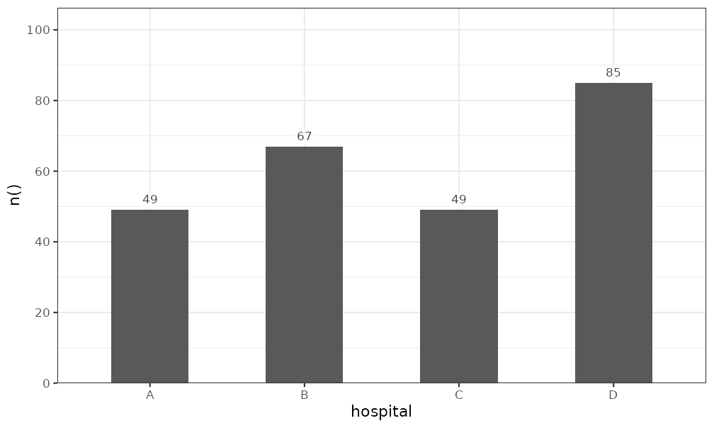
plot2() applies theme_minimal2() by default. This theme is based on ggplot2::theme_minimal(), with fewer grid lines, more white space and the legend at the top, and it is suited to print. The theme argument sets another theme, and theme = NULL uses the default theme of ggplot2:

admitted_patients |>
  plot2(x = hospital, y = n(), theme = ggplot2::theme_bw())

A partial theme, made with ggplot2::theme(), is added to theme_minimal2(), so that only the given elements change:

admitted_patients |>
  plot2(x = hospital,
        y = n(),
        theme = ggplot2::theme(panel.grid.major.y = ggplot2::element_blank()))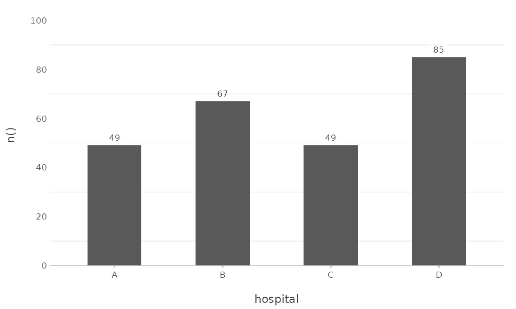

Other arguments change frequent elements directly. background sets the background colour, text_factor scales all text, and legend.position places the legend:

admitted_patients |>
  plot2(x = hospital,
        y = n(),
        category = gender,
        background = "#F5F5F0",
        text_factor = 1.2,
        legend.position = "right")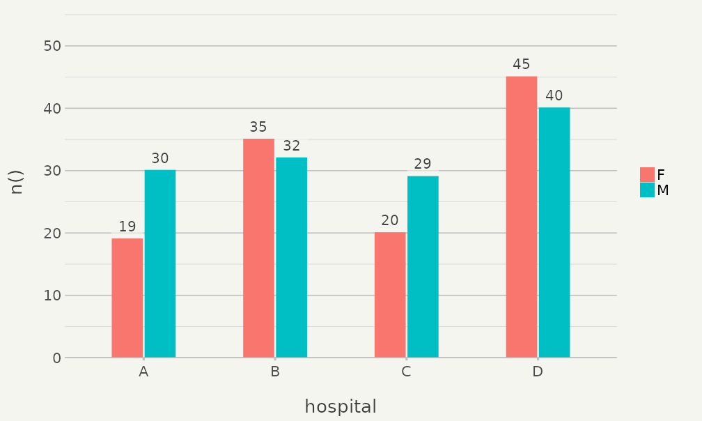

The options plot2.theme, plot2.colour_background, plot2.text_factor, plot2.colour_font_primary (title), plot2.colour_font_secondary (subtitle and caption) and plot2.colour_font_axis (axis titles) set these defaults for all plots. ?plot2-options lists all options.

Titles

Titles support markdown for italic (*text*) and bold (**text**) text, which is often needed for the names of species, and <br> for a line break. plot2() converts the markdown to a plotmath expression with md_to_expression():

data.frame(species = c("E. coli", "K. pneumoniae", "S. aureus"),
           isolates = c(412, 128, 197)) |>
  plot2(x = species,
        y = isolates,
        title = "Isolates of *E. coli*, *K. pneumoniae* and *S. aureus*",
        subtitle = "**Fictitious** data",
        x.label_italic = TRUE)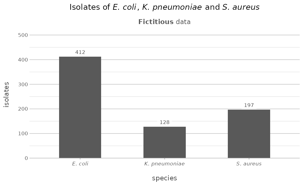

Set markdown = FALSE to show the text as it is. Long titles are wrapped at title.linelength characters.