The following plot types are supported.
Any ggplot2 geom is supported, but we added support for
some other, more advanced plots.
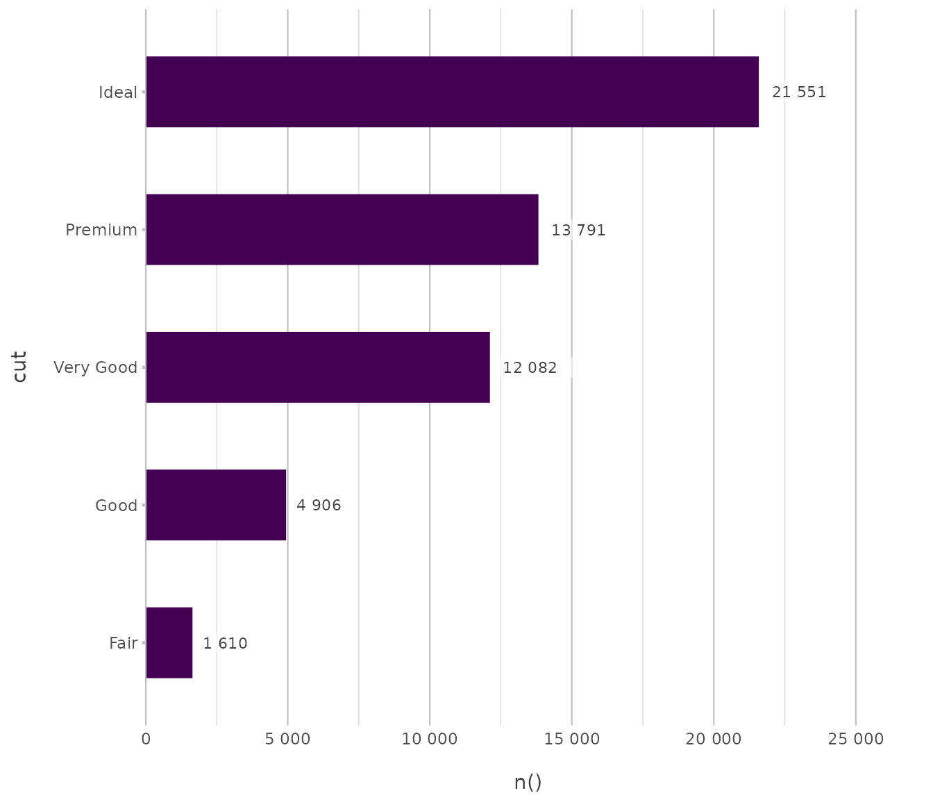
Column / Bar
Used for comparing discrete categories through rectangular bars.
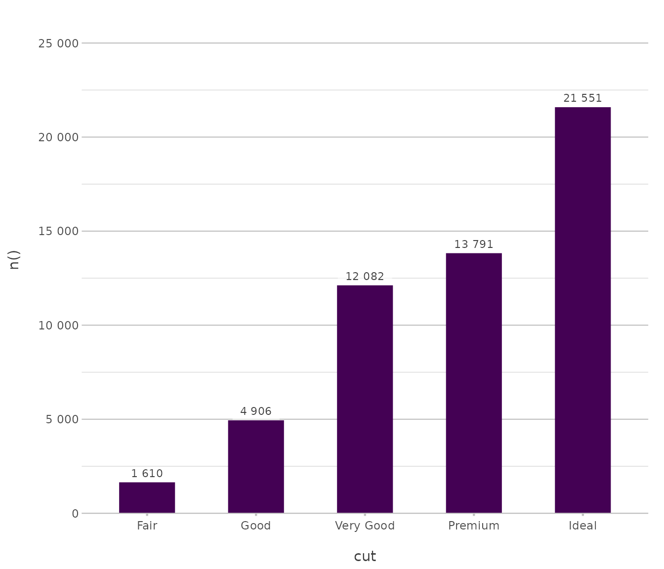
In plot2, bar types are horizontal alternatives for
column types (just like MS Excel):
Line
Used for visualising trends over ordered intervals.
pressure |> # from base R
  plot2(x = temperature,
        y = pressure,
        type = "line")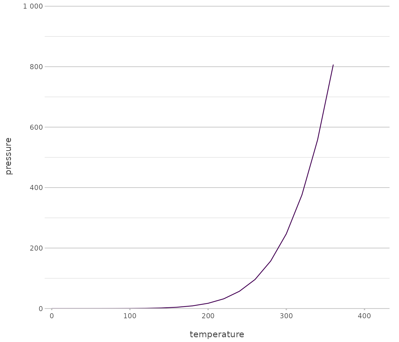
pressure |>
  plot2(x = temperature,
        y = pressure,
        type = "line-point")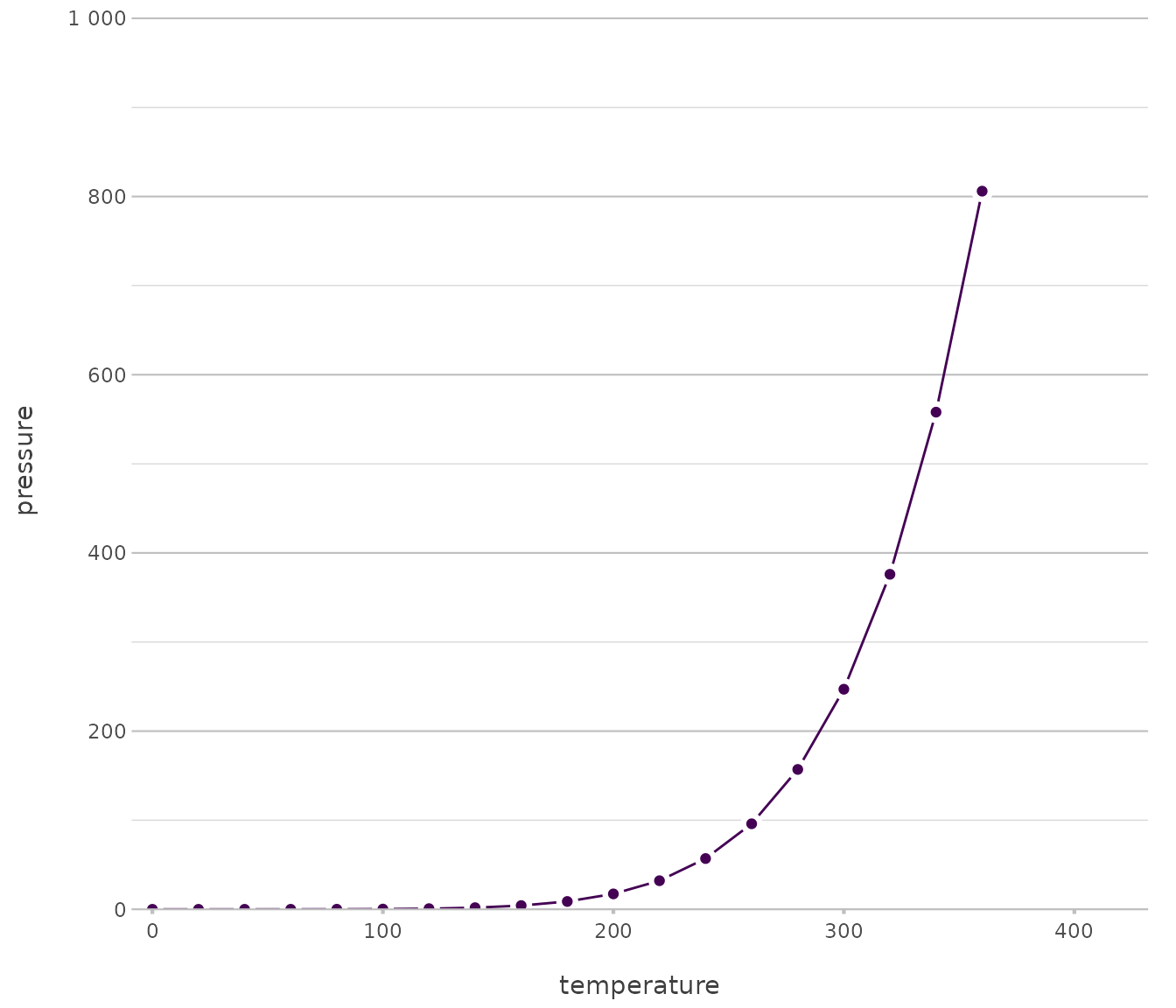
Point
Used for displaying individual observations in a two dimensional space.
iris |> # from base R
  plot2()
#> ℹ Using category = Species
#> ℹ Using type = "point" since both axes are numeric
#> ℹ Using x = Sepal.Length
#> ℹ Using y = Sepal.Width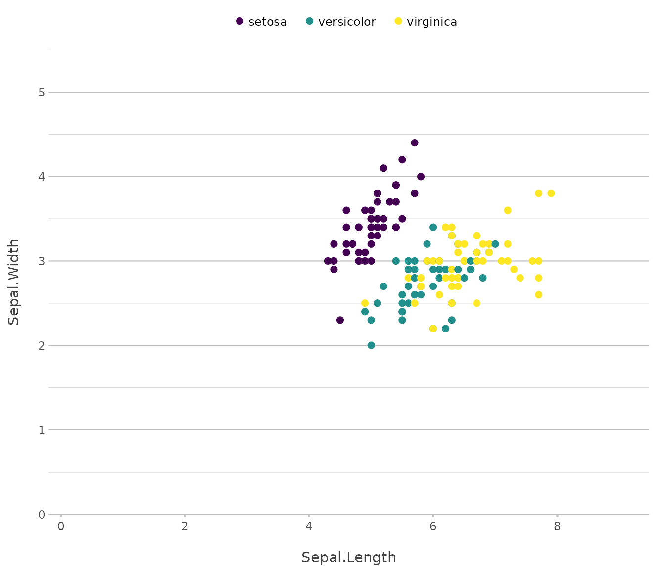
diamonds |>
  plot2(x = carat,
        y = price,
        category = cut,
        type = "point")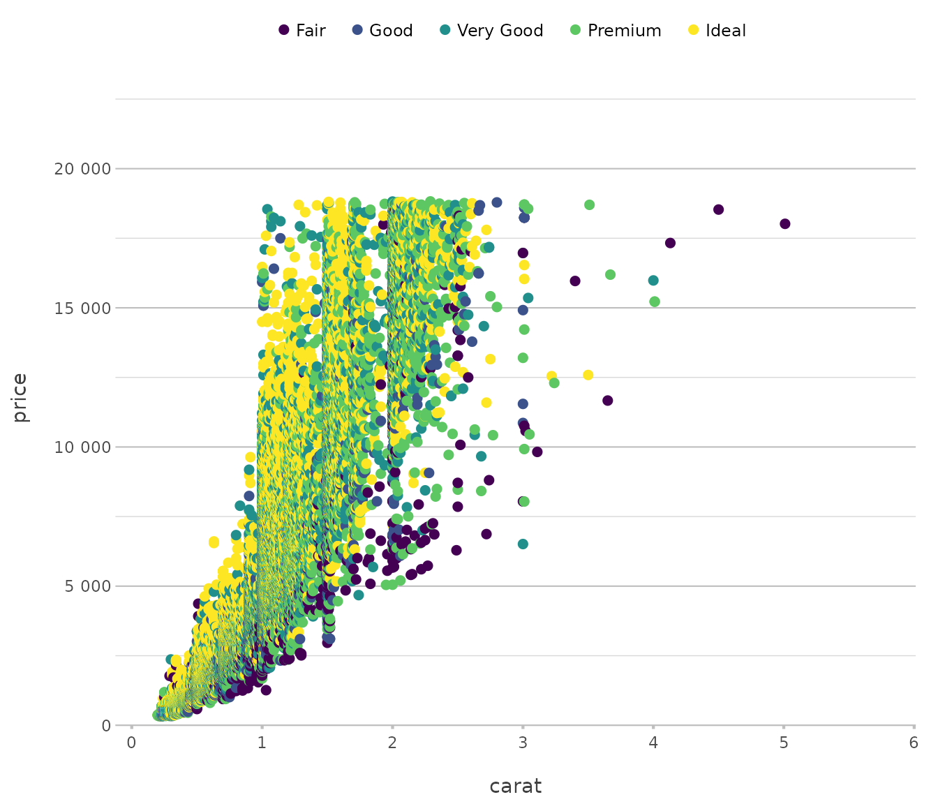
Area
Used for emphasising cumulative magnitudes across continuous domains.
pressure |>
  plot2(x = temperature,
        y = pressure,
        type = "area")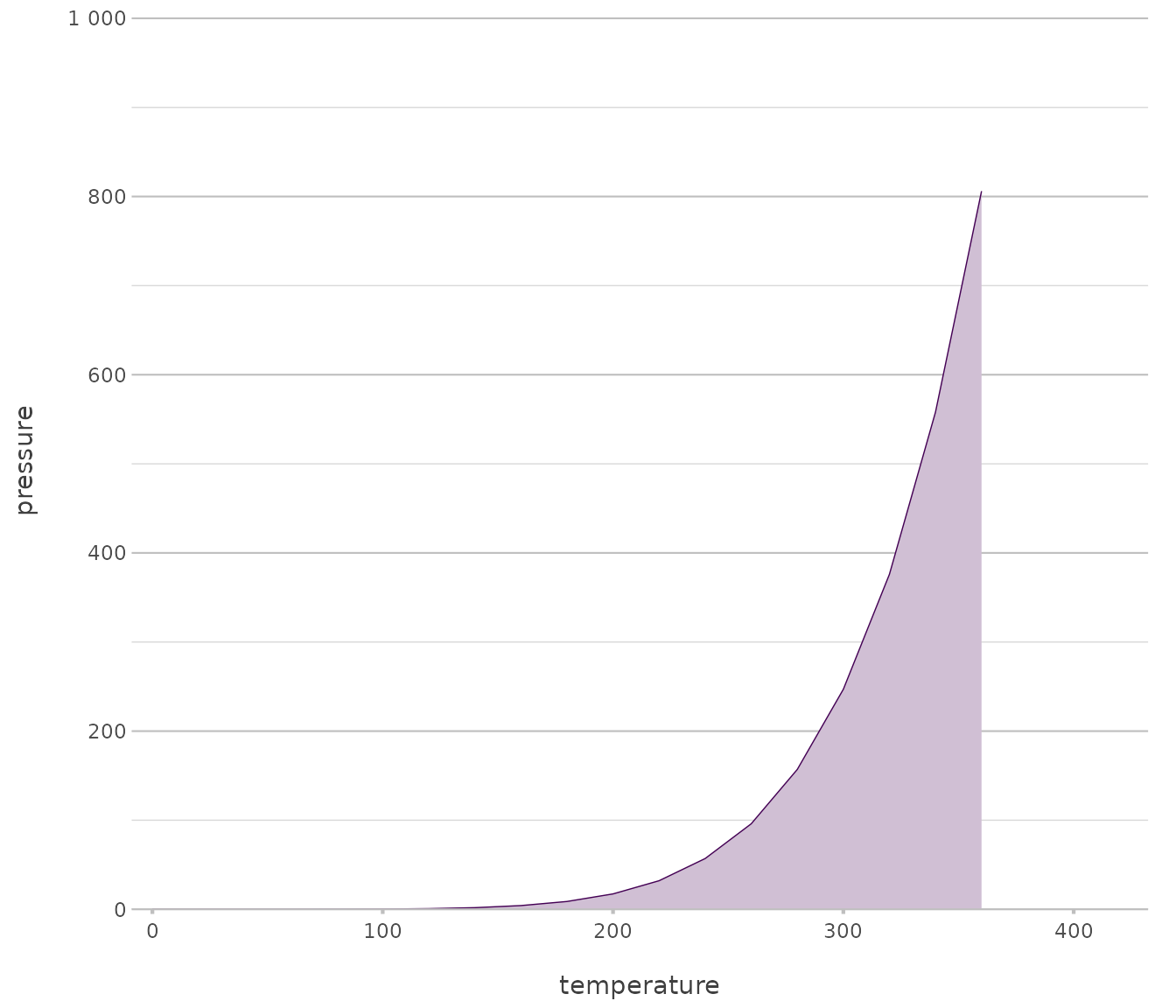
airquality |>
  plot2(x = Day,
        y = Wind,
        category = Month,
        category.character = TRUE,
        stacked_fill= TRUE,
        type = "area")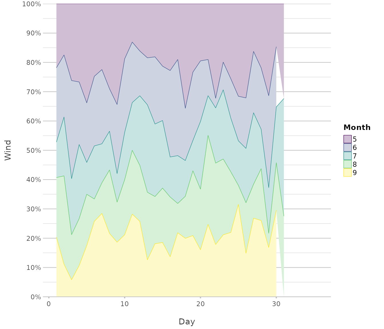
Boxplot / Violin
Used for summarising and comparing distributions with focus on spread and density.
iris |>
  plot2(x = Species,
        type = "violin")
#> ℹ Using y = Sepal.Length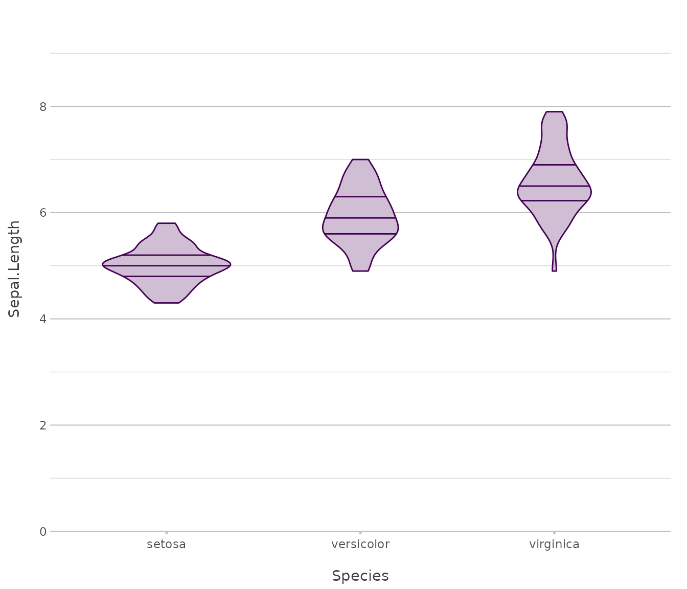
iris |>
  plot2(x = Species,
        y = where(is.double),
        type = "boxplot")
#> ℹ Using y = c(Petal.Length, Petal.Width, Sepal.Length, Sepal.Width)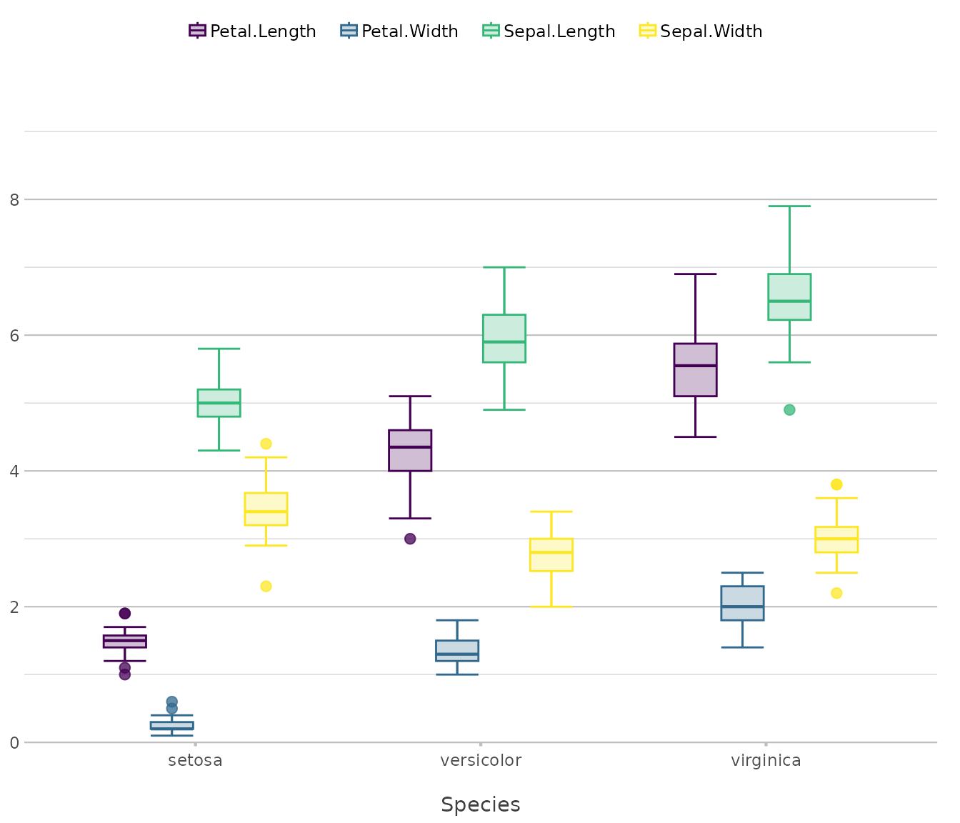
Histogram
Used for visualising the frequency distribution of continuous variables.
diamonds |>
  plot2(x = price,
        type = "hist")
#> ℹ Assuming smooth = TRUE for type = "histogram"
#> ℹ Using binwidth = 841 based on data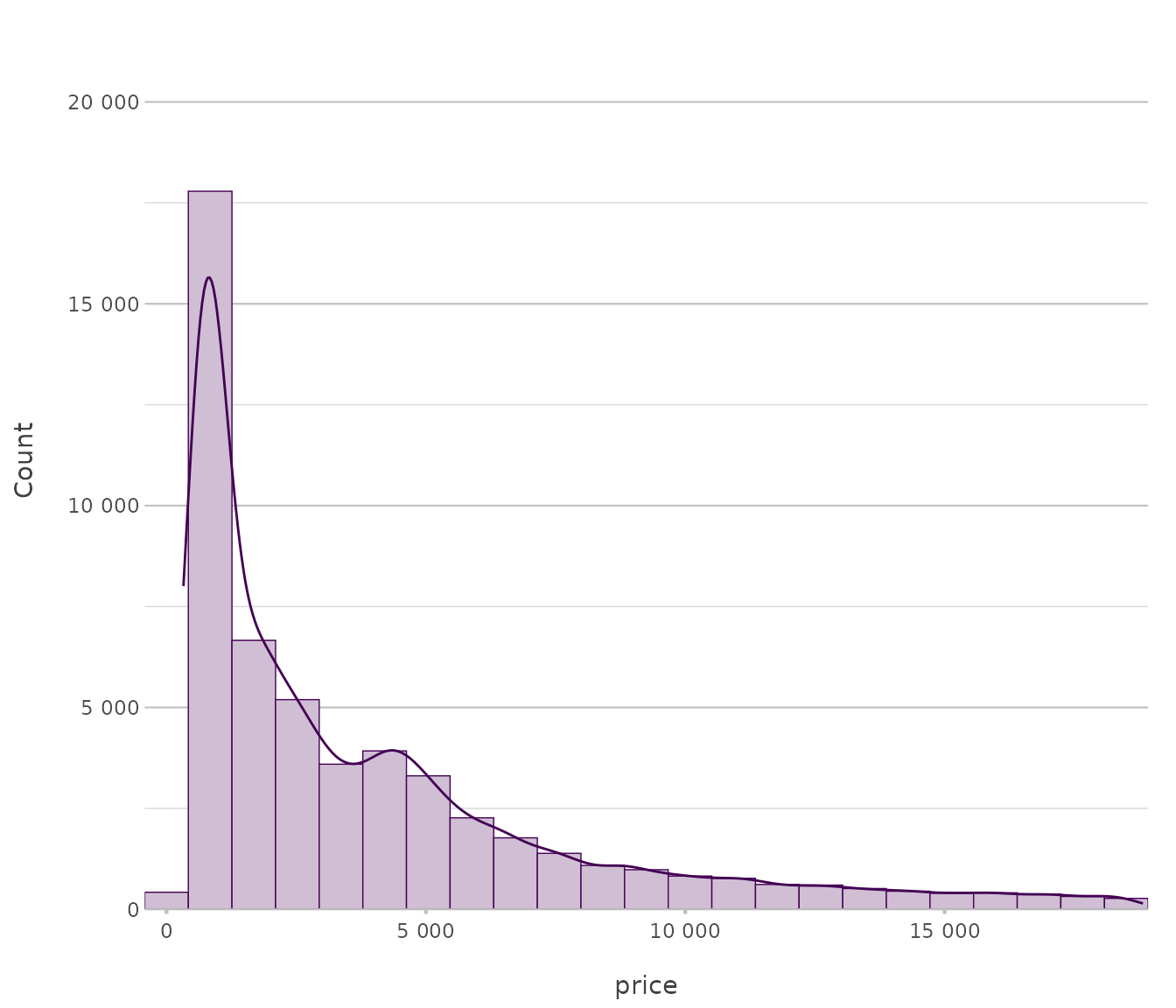
Geo (sf)
Used for mapping spatial data encoded as simple features.
netherlands |> # from this plot2 package
  plot2()
#> ℹ Assuming datalabels.centroid = TRUE. Set to FALSE for a point-on-surface
#> placing of datalabels.
#> ℹ Using category = area_km2
#> ℹ Using datalabels = province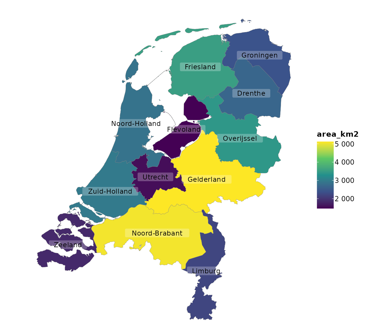
Beeswarm
Used for showing distributions of individual observations without overlap.
iris |>
  plot2(x = Species,
        y = Sepal.Length,
        type = "beeswarm")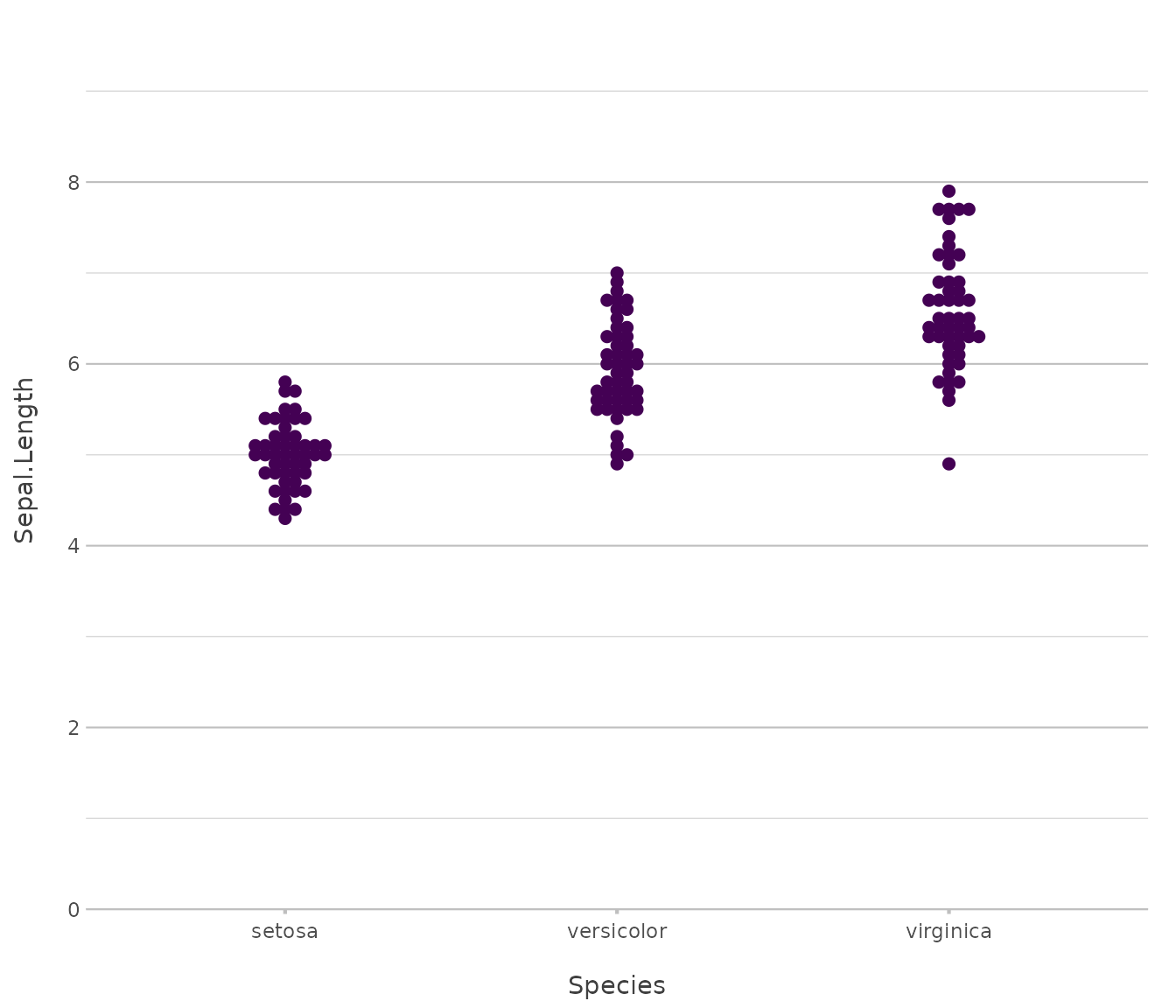
Back-to-back
Used for contrasting two mirrored groups across shared categories.
admitted_patients |> # from this plot2 package
  plot2(x = age_group,
        y = n(),
        facet = ward,
        type = "back-to-back")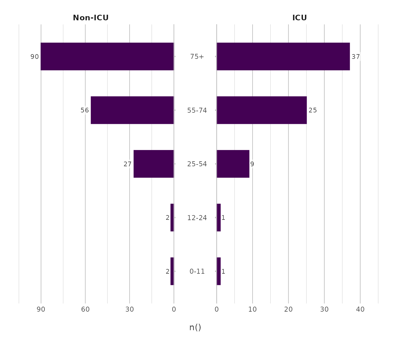
admitted_patients |> # from this plot2 package
  plot2(x = age_group,
        y = n(),
        y.limits = c(0, 60),
        category = gender,
        facet = ward,
        type = "back-to-back")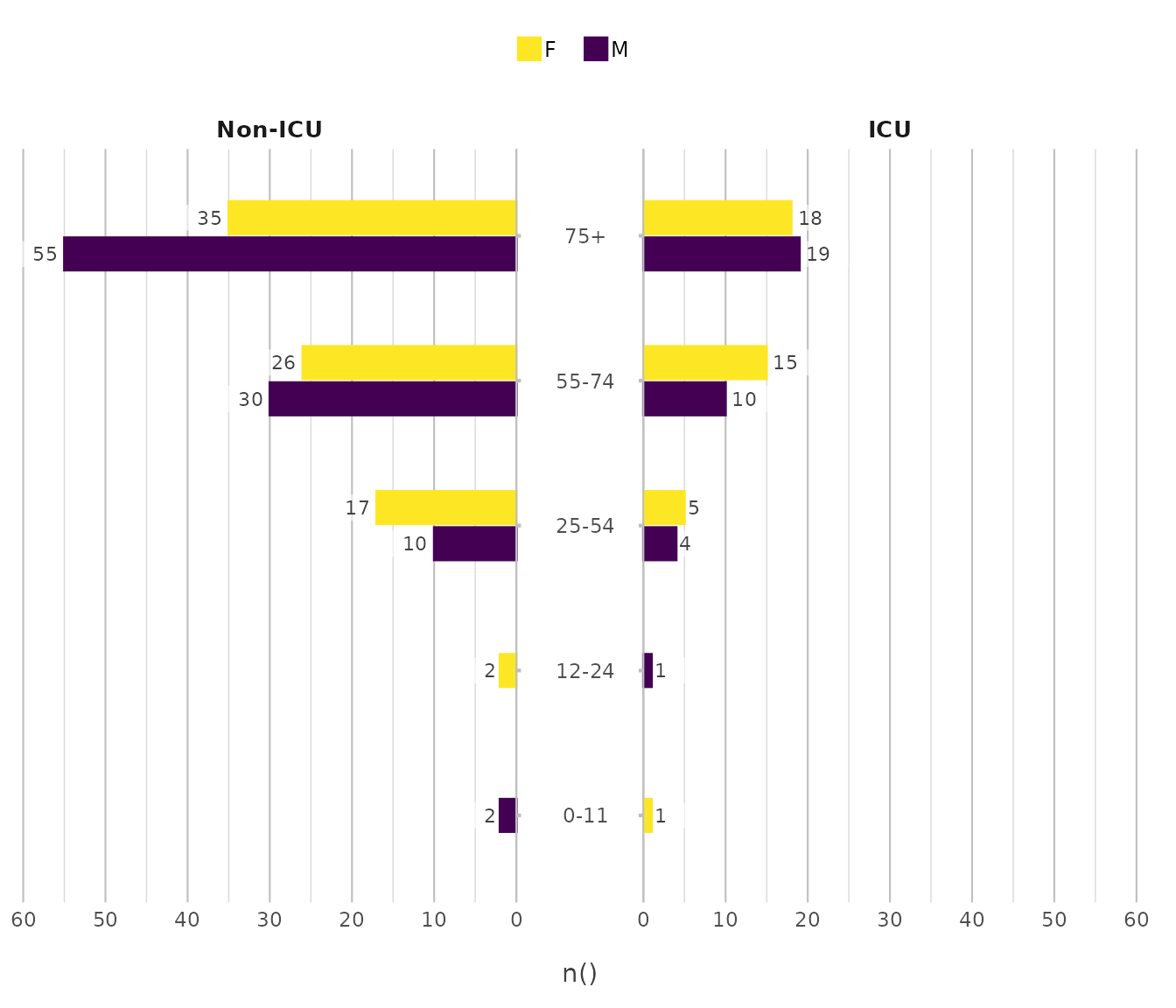
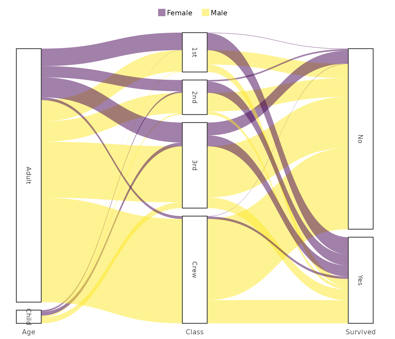
Sankey
Used for depicting flows or transitions between connected stages.
Titanic |> # from base R
  plot2(x = c(Age, Class, Survived),
        category = Sex,
        type = "sankey")
#> ℹ Assuming sankey.remove_axes = TRUE
#> ! Input class 'table' was transformed using `as.data.frame()`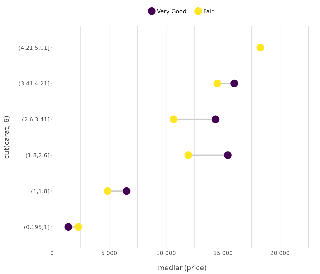
Spider
Used for comparing multivariate values across categorical axes arranged radially, enabling pattern recognition and relative magnitude assessment between groups.
# spider plots can have a filling colour, but it's hardly ever useful
diamonds |>
    plot2(x = cut,
          y = mean(price),
          category = color,
          type = "spider",
          y.labels = dollars,
          colour_fill = "viridis")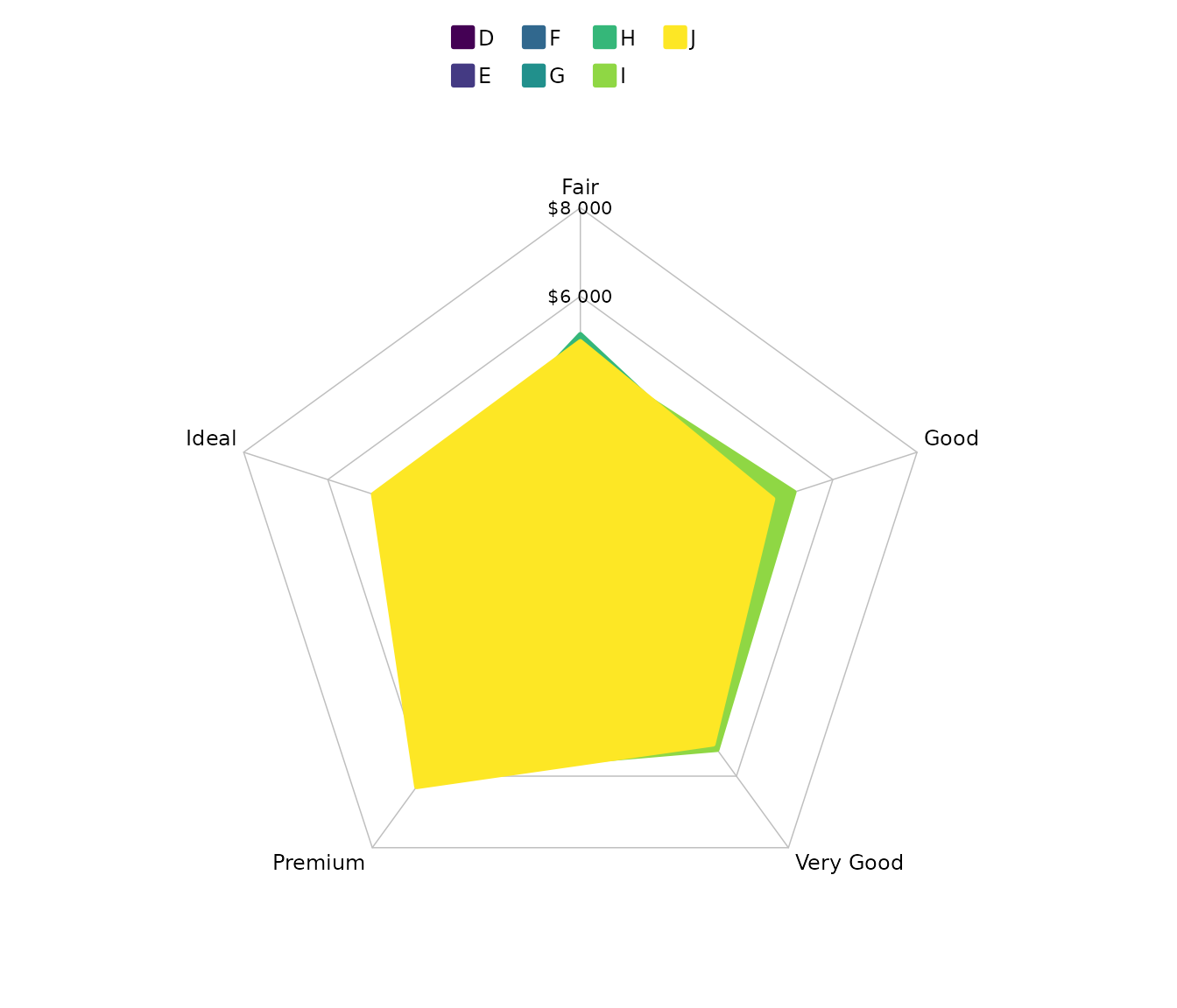
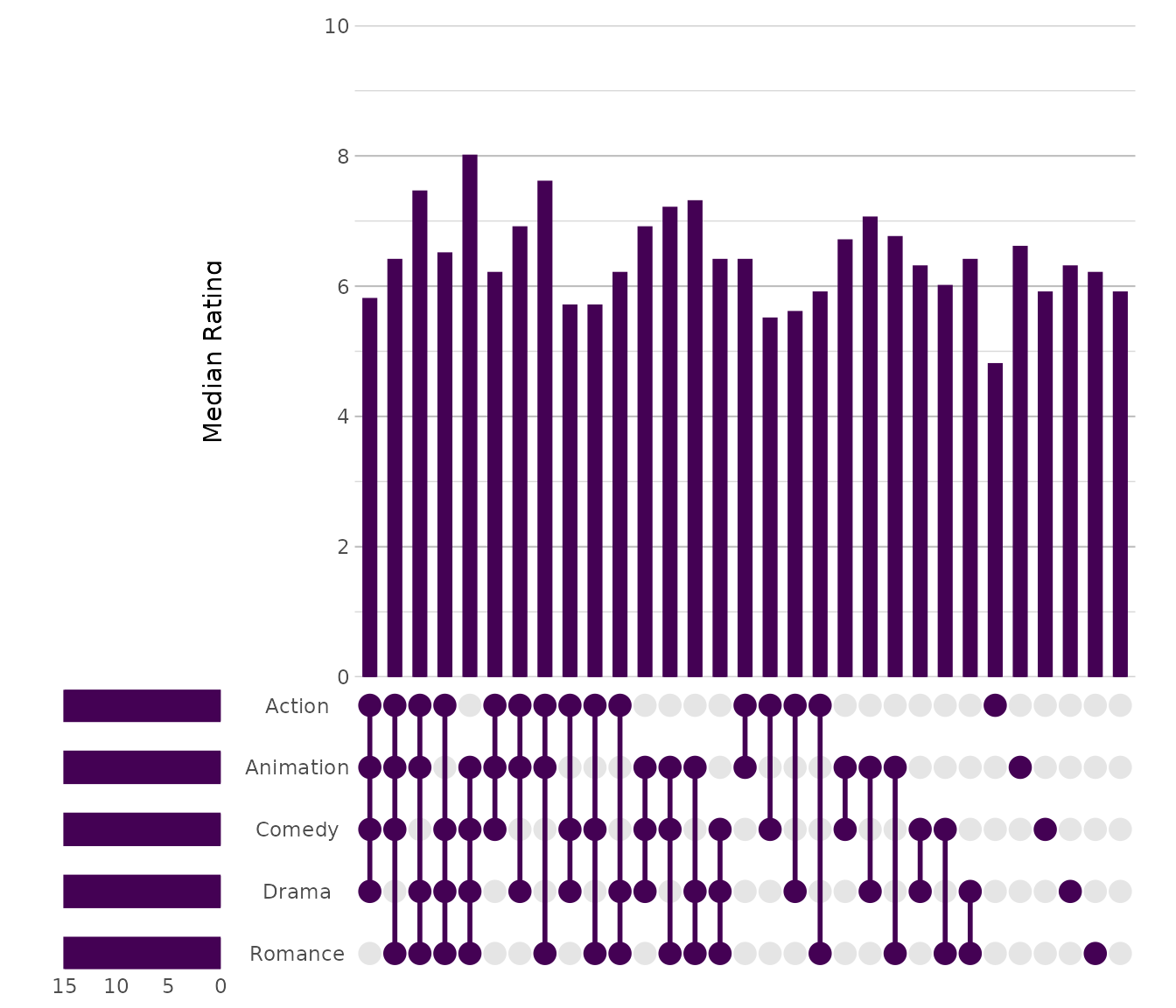
UpSet
Used for analysing intersections among multiple sets with scalable clarity.
movies |> # from the ggplot2movies package
  plot2(x = c(Action, Animation, Comedy, Drama, Romance),
        type = "upset")
#> ℹ Using summarise_function = sum for UpSet plot
#> ℹ Using y = 1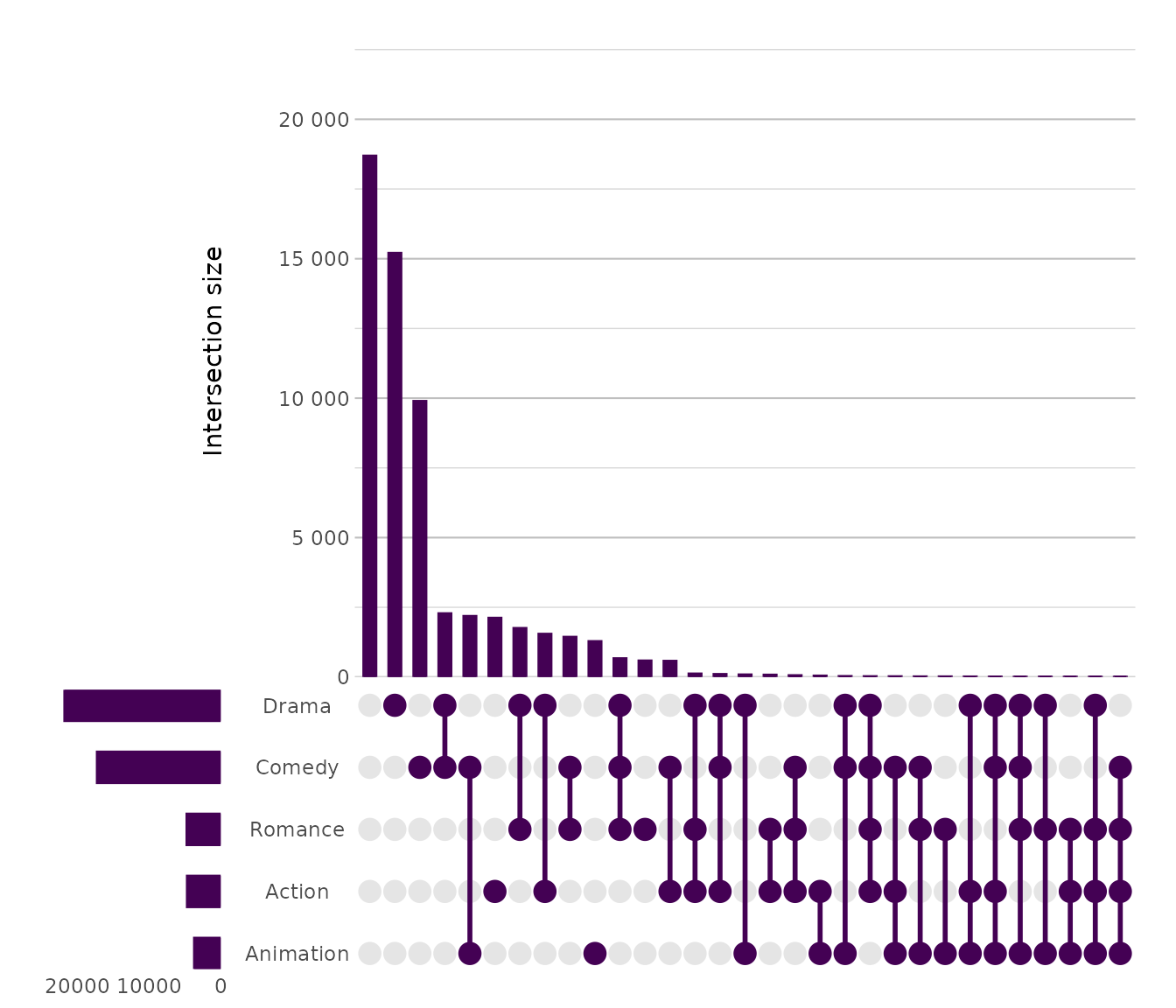
movies |>
  plot2(x = c(Action, Animation, Comedy, Drama, Romance),
        y = median(rating),
        y.title = "Median Rating",
        x.sort = TRUE,
        type = "upset")
#> ℹ Using summarise_function = sum for UpSet plot