How to predict antimicrobial resistance • AMR (for R)

Needed R packages

As with many uses in R, we need some additional packages for AMR data analysis. Our package works closely together with the tidyverse packages dplyr and ggplot2. The tidyverse tremendously improves the way we conduct data science - it allows for a very natural way of writing syntaxes and creating beautiful plots in R.

Our AMR package depends on these packages and even extends their use and functions.

library(dplyr)
#> Error in get(paste0(generic, ".", class), envir = get_method_env()) : 
#>   object 'type_sum.accel' not found
library(ggplot2)
library(AMR)

# (if not yet installed, install with:)
# install.packages(c("tidyverse", "AMR"))

Prediction analysis

Our package contains a function resistance_predict(), which takes the same input as functions for other AMR data analysis. Based on a date column, it calculates cases per year and uses a regression model to predict antimicrobial resistance.

It is basically as easy as:

# resistance prediction of piperacillin/tazobactam (TZP):
resistance_predict(tbl = example_isolates, col_date = "date", col_ab = "TZP", model = "binomial")

# or:
example_isolates %>%
  resistance_predict(
    col_ab = "TZP",
    model = "binomial"
  )

# to bind it to object 'predict_TZP' for example:
predict_TZP <- example_isolates %>%
  resistance_predict(
    col_ab = "TZP",
    model = "binomial"
  )

The function will look for a date column itself if col_date is not set.

When running any of these commands, a summary of the regression model will be printed unless using resistance_predict(..., info = FALSE).

This text is only a printed summary - the actual result (output) of the function is a data.frame containing for each year: the number of observations, the actual observed resistance, the estimated resistance and the standard error below and above the estimation:

predict_TZP
#> # A tibble: 33 × 7
#>     year  value se_min se_max observations observed estimated
#>  * <dbl>  <dbl>  <dbl>  <dbl>        <int>    <dbl>     <dbl>
#>  1  2002 0.2        NA     NA           15   0.2       0.0562
#>  2  2003 0.0625     NA     NA           32   0.0625    0.0616
#>  3  2004 0.0854     NA     NA           82   0.0854    0.0676
#>  4  2005 0.05       NA     NA           60   0.05      0.0741
#>  5  2006 0.0508     NA     NA           59   0.0508    0.0812
#>  6  2007 0.121      NA     NA           66   0.121     0.0889
#>  7  2008 0.0417     NA     NA           72   0.0417    0.0972
#>  8  2009 0.0164     NA     NA           61   0.0164    0.106 
#>  9  2010 0.0566     NA     NA           53   0.0566    0.116 
#> 10  2011 0.183      NA     NA           93   0.183     0.127 
#> # ℹ 23 more rows

The function plot is available in base R, and can be extended by other packages to depend the output based on the type of input. We extended its function to cope with resistance predictions:

plot(predict_TZP)

This is the fastest way to plot the result. It automatically adds the right axes, error bars, titles, number of available observations and type of model.

We also support the ggplot2 package with our custom function ggplot_sir_predict() to create more appealing plots:

ggplot_sir_predict(predict_TZP)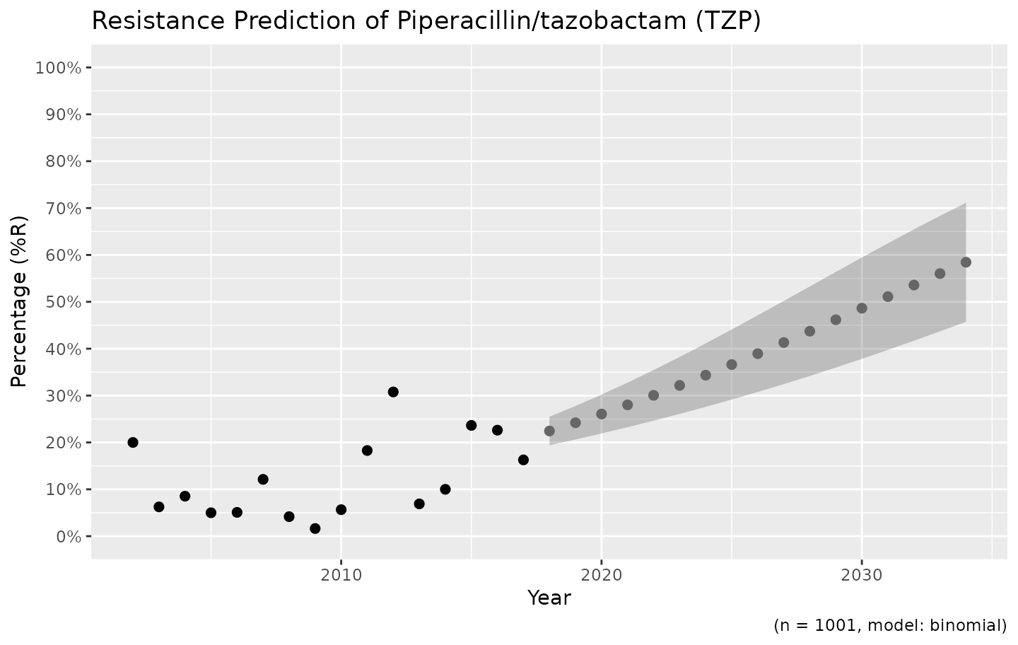


# choose for error bars instead of a ribbon
ggplot_sir_predict(predict_TZP, ribbon = FALSE)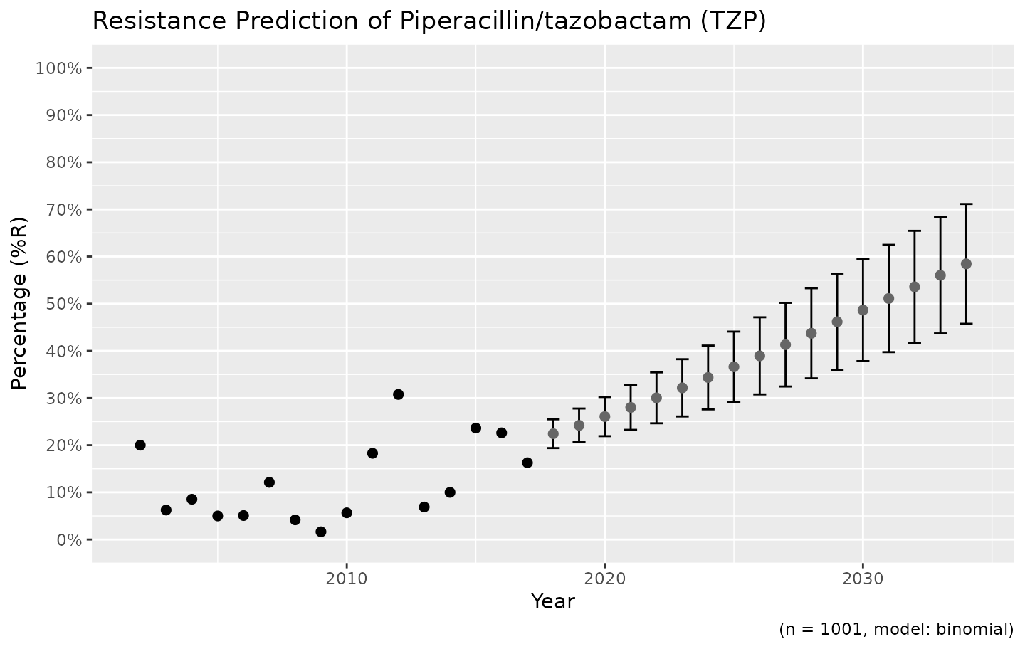

Choosing the right model

Resistance is not easily predicted; if we look at vancomycin resistance in Gram-positive bacteria, the spread (i.e. standard error) is enormous:

example_isolates %>%
  filter(mo_gramstain(mo, language = NULL) == "Gram-positive") %>%
  resistance_predict(col_ab = "VAN", year_min = 2010, info = FALSE, model = "binomial") %>%
  ggplot_sir_predict()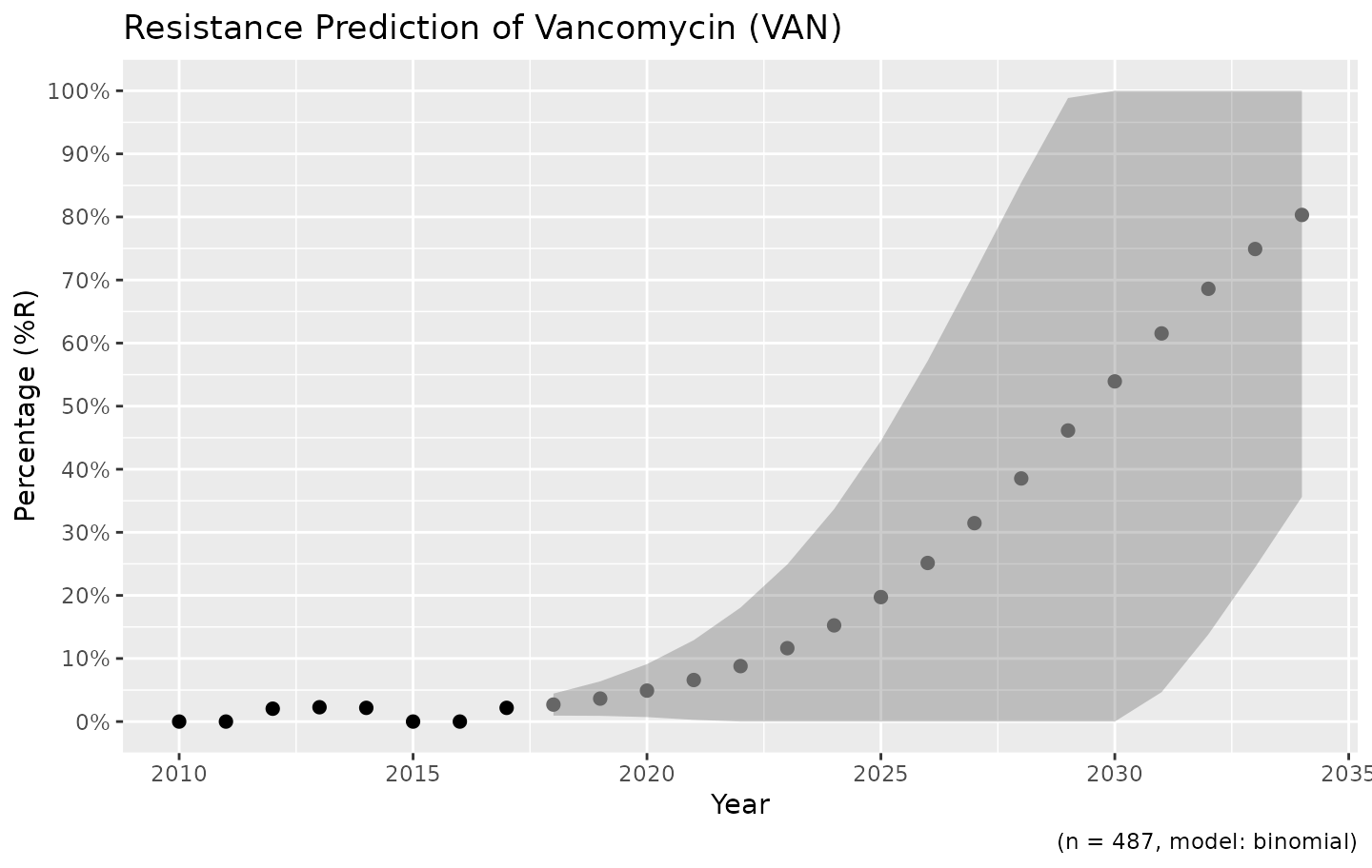

Vancomycin resistance could be 100% in ten years, but might remain very low.

You can define the model with the model parameter. The model chosen above is a generalised linear regression model using a binomial distribution, assuming that a period of zero resistance was followed by a period of increasing resistance leading slowly to more and more resistance.

Valid values are:

Input values	Function used by R	Type of model
`"binomial"` or `"binom"` or `"logit"`	`glm(..., family = binomial)`	Generalised linear model with binomial distribution
`"loglin"` or `"poisson"`	`glm(..., family = poisson)`	Generalised linear model with poisson distribution
`"lin"` or `"linear"`	`lm()`	Linear model

For the vancomycin resistance in Gram-positive bacteria, a linear model might be more appropriate:

example_isolates %>%
  filter(mo_gramstain(mo, language = NULL) == "Gram-positive") %>%
  resistance_predict(col_ab = "VAN", year_min = 2010, info = FALSE, model = "linear") %>%
  ggplot_sir_predict()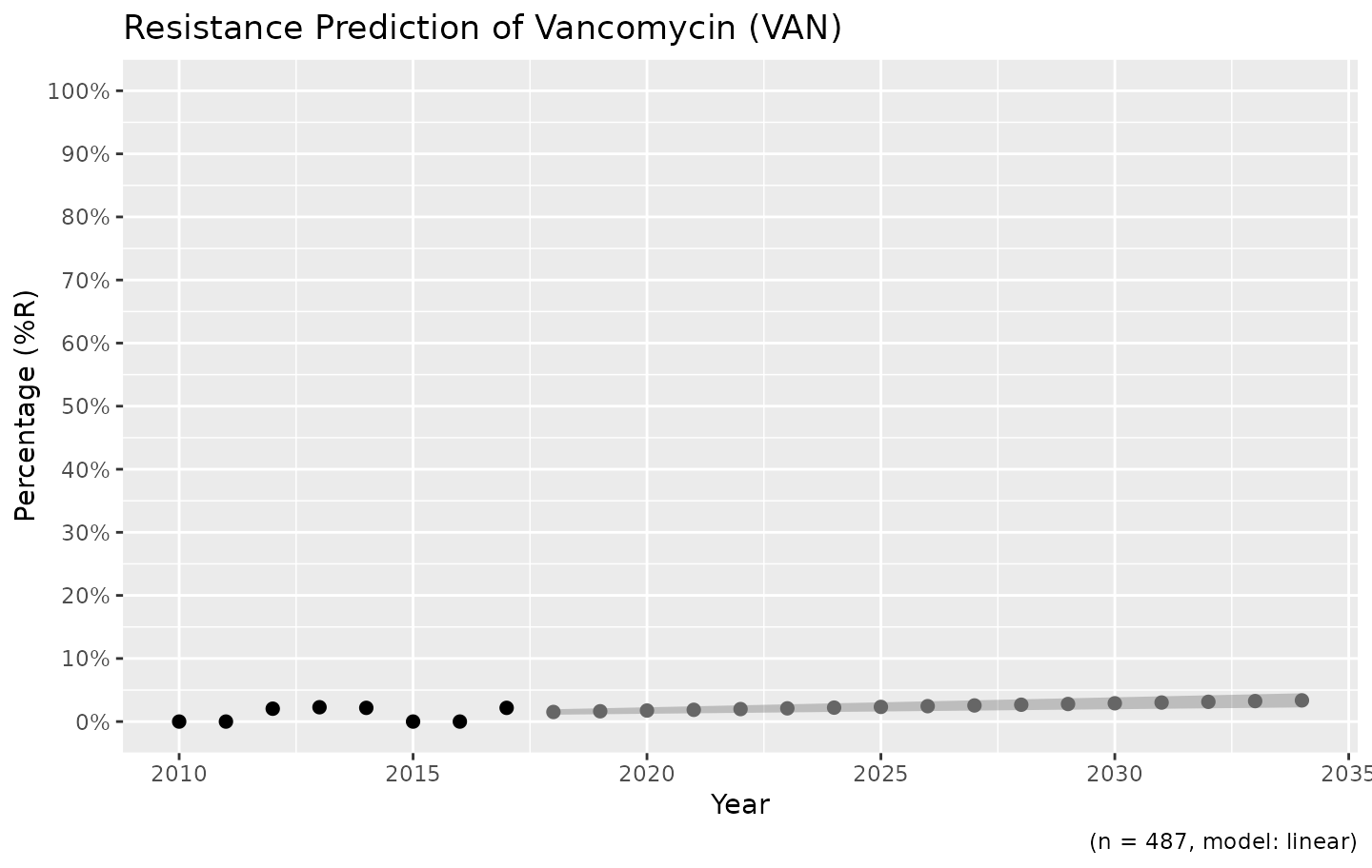

The model itself is also available from the object, as an attribute:

model <- attributes(predict_TZP)$model

summary(model)$family
#> 
#> Family: binomial 
#> Link function: logit

summary(model)$coefficients
#>                  Estimate  Std. Error   z value     Pr(>|z|)
#> (Intercept) -200.67944891 46.17315349 -4.346237 1.384932e-05
#> year           0.09883005  0.02295317  4.305725 1.664395e-05